Move the Hand, Not Every Joint: Why Inverse Kinematics Makes Robots Easier to Control
Inverse kinematics turns a desired gripper pose into the joint angles needed to reach it, separating the task a robot should perform from the motor coordinates used to perform it.
Inverse kinematics solves the translation problem between task space and joint space.
A robot arm is generally a chain of motors where software talks to it in joint angles. Because angles are the only thing the motors can actually do, every task you care about is expressed the other way around, as a position in space: pick up the cup at this spot on the table, hold the camera here, place the screw on that hole. Somewhere between the task and the motors, "put the gripper at (x, y, z)" has to become "rotate joint 1 to 42 degrees, joint 2 to negative 13, joint 3 to 77". Inverse kinematics is that translation step.
Those two vocabularies have names, and they come up constantly in robotics. Joint space is the robot's internal coordinate system, with one number per motor. A pose for the four-joint demo arm below is just a list of angles like (42°, -13°, 77°, 5°), and the arm's controller only ever consumes lists like that. Task space (often called Cartesian space) is the coordinate system the work is described in: positions and orientations out in the world, measured in meters and directions, the same x, y, z you would use to say where the cup sits on the table. You, your sensors, and your task planner all think in task space. The motors only understand joint space. Inverse kinematics is the bridge from the first to the second.
The name makes sense once you see its mirror image. Forward kinematics (FK) goes from angles to position. Given every joint angle and the length of every link, you can chain the transforms together and compute exactly where the gripper ends up. That direction is easy, deterministic, and has one answer. Writing the pose of the end of the arm (a pose is a position plus an orientation, and the word means that everywhere in robotics) as a function of the joint angles:
Inverse kinematics runs the arrow backwards. You know the target pose and you want joint angles that produce it:
That innocent little superscript hides all the trouble. The function is a stack of trigonometry, so inverting it is a nonlinear problem. It can have many solutions (reach the same cup with your elbow up or your elbow down), exactly one, or none at all when the target is out of reach. For most arms beyond a few joints there is no clean formula for , which is why the field has spent forty years inventing solvers for it.
Feel the problem: no IK
Without IK, an operator controls the base, shoulder, elbow, and wrist directly, much like the jog controls on an industrial teach pendant.
Every joint moves the links after it, turning a Cartesian target into manual optimization. The operator becomes the solver, which scales poorly beyond a small arm.
Now with IK
With IK, the target is specified in task space and the solver recomputes the joint angles every frame. An unreachable target produces the closest pose allowed by the arm's reach and joint limits.
The goal stays in task space while the solver handles joint space.
The solver behind this demo is cyclic coordinate descent (CCD), one of the simplest IK algorithms that actually works. It loops over the joints from the wrist back to the base, and rotates each one, on its own axis, by whatever angle best swings the gripper toward the target. One sweep helps a little; repeated sweeps converge. This demo runs 18 sweeps per frame with a cap on how far any joint can move per step, plus per-joint angle limits so the arm can't fold through itself. That is the whole algorithm. It's the same iterate-and-improve loop you were doing by hand in the first scene, executed a few thousand times faster and without complaints.
Why IK matters even with AI
IK sits in the middle of almost everything a robot does with its body, usually invisibly:
- Manipulation. A grasp planner outputs "gripper here, oriented like this". IK turns each candidate grasp into joint angles, and grasps with no IK solution get discarded before anything moves.
- Motion planning. Planners like the ones in MoveIt plan through joint space, but their start and goal states usually arrive as Cartesian poses. IK converts them. Path constraints like "keep the cup upright while carrying it" get enforced by solving IK repeatedly along the path.
- Teleoperation and data collection. When an operator steers a robot with a controller or their own tracked hands, their input is a stream of target poses. IK maps that stream onto the robot's joints in real time. Every teleop demonstration dataset behind today's manipulation models was collected through an IK layer.
- Legged robots. A quadruped or humanoid places its feet at planned positions on the ground. Each footstep is an IK problem for that leg, solved every control cycle while the body moves.
- Animation and simulation. Game engines and animation tools use IK to pin feet to terrain and hands to objects. The math is identical, which is why graphics papers and robotics papers cite each other constantly.
There's also a subtler reason IK earns its keep. Joint space and task space disagree about distance. Two arm poses can be millimeters apart at the gripper and far apart in joint angles, or the reverse. Humans, tasks, and sensors all live in task space. Motors live in joint space. Any system where those two meet needs the translation, and it needs it fast enough to run inside a control loop.
The technique landscape
Solvers fall into a few families, and each one trades generality against speed against robustness.
Closed-form (analytic) solutions
For specific arm geometries you can invert symbolically and get exact answers in microseconds, with every solution enumerated. Most six-axis industrial arms are deliberately designed with a spherical wrist (three axes intersecting at a point) so that position and orientation decouple and a closed-form solution exists. The best known tool here is IKFast from Rosen Diankov's OpenRAVE work, which generates analytic solver code for a given robot automatically. When your robot admits one, an analytic solver is the fastest and most reliable option, full stop. The limitation is rigidity: add a joint, change the geometry, or ask for a redundant arm (one with more joints than the task strictly needs), and the closed form stops existing.
Jacobian methods
The workhorse family. The Jacobian matrix tells you how small joint velocities map to small gripper velocities. Invert that relationship locally and you can walk the arm toward a target step by step. Three classic variants, laid out cleanly in Buss's tutorial survey:
- Jacobian transpose uses instead of a true inverse. Cheap and stable, but takes crude steps.
- Pseudoinverse uses the Moore-Penrose inverse for locally optimal steps, and the leftover freedom of a redundant arm can be spent on secondary goals like staying away from joint limits. Its weakness is violent behavior near singularities, the configurations where the arm loses a direction of motion (think of a fully straightened elbow).
- Damped least squares (DLS), introduced independently by Wampler and Nakamura and Hanafusa in 1986, adds a damping term that sacrifices a little accuracy for stability near singularities. This is the default serious choice in the family.
Jacobian solvers are general (any chain, any joint count) and integrate naturally with velocity control, which is why differential IK (solving for a small velocity step each control tick instead of a full pose) runs inside many real-time controllers today.
Simple geometric solvers: CCD and FABRIK
These skip the Jacobian entirely in favor of intuitive geometric rules applied over and over until the pose settles. CCD, formalized for manipulators by Wang and Chen in 1991, is what the second demo above runs: rotate one joint at a time to best align the end effector (the robotics term for the gripper, hand, or tool at the end of the chain) with the target, repeat. FABRIK, published by Aristidou and Lasenby in 2011, works on joint positions instead of angles. It slides points along the chain in a forward pass and a backward pass until they settle, which produces smoother poses than CCD and converges quickly without any trigonometry in the inner loop. Both are simple to implement, fast, and tolerant of joint limits bolted on as clamps. They dominate games and animation, and FABRIK has crossed into robotics for many-jointed arms and continuum robots (snake-like designs that bend along their whole body instead of at distinct joints). The 2018 survey by Aristidou, Lasenby, Chrysanthou, and Shamir covers this whole family and is the best single entry point to the literature.
Optimization-based solvers
Treat IK as a constrained optimization problem: minimize distance to the target pose subject to joint limits, collision avoidance, or whatever else you can express as a cost or constraint. TRAC-IK, from Beeson and Ames in 2015, is the well-known open-source example. It runs an improved Newton-style solver and a sequential quadratic programming solver (a standard numerical optimization method) concurrently and takes whichever finishes first. That fixed a chronic weakness of the older KDL solver on humanoid arms, which often reported no solution even when one existed. Modern humanoid and legged-robot stacks push this further, phrasing whole-body IK as one big optimization problem (a quadratic program) that juggles balance, contact, and reach targets at once, solved at hundreds or thousands of hertz.
Learning-based solvers
Neural networks can learn the inverse map directly, and recent work like IKFlow uses normalizing flows (a type of neural network that can be run backwards as easily as forwards) to generate the full diverse set of solutions for redundant arms in one shot rather than one solution at a time. Learned IK also shows up implicitly: end-to-end manipulation policies that output joint actions from camera images have effectively absorbed an IK layer into the network. Explicit learned solvers remain more of a research frontier than a production default, but the direction is active.
What robots actually use today
In practice the choices are boring and sensible. Industrial six-axis arms use analytic solvers, often IKFast-generated, because the geometry allows it and the determinism is worth it. ROS and MoveIt users overwhelmingly configure TRAC-IK or the stock KDL solver for general arms. Real-time control loops and teleop stacks run damped-least-squares differential IK. Humanoids and quadrupeds run optimization-based whole-body solvers. Games and character animation run FABRIK and CCD. Pick the simplest thing that fits your robot's shape and your latency budget, and it's usually one of these five answers.
Where this fits for edge robotics
Everything in the two demos above, from the CCD loop to the joint-limit clamps, is a few hundred lines of TypeScript running at 60 frames per second in your browser tab. The same math scales down comfortably to a control loop on a Jetson Orin Nano or a Raspberry Pi sitting inside an arm. That's the layer we care about at Wendy: the solver is standard, published math, and the hard part is shipping and updating it on a fleet of devices like any other piece of software. On WendyOS, an IK-driven controller is just an app you deploy with wendy run, next to your camera pipeline and your policy model.
If you got the arm to touch the target in the first scene, you have manually performed cyclic coordinate descent, and the second scene will forever feel like cheating. That feeling is the last forty years of robotics working as intended.
Sources
- Samuel R. Buss. Introduction to Inverse Kinematics with Jacobian Transpose, Pseudoinverse and Damped Least Squares Methods. Tutorial survey, UC San Diego, 2004.
- L.-C. T. Wang and C. C. Chen. A Combined Optimization Method for Solving the Inverse Kinematics Problem of Mechanical Manipulators. IEEE Transactions on Robotics and Automation, 7(4), 1991. The standard reference for CCD on manipulators.
- C. W. Wampler. Manipulator Inverse Kinematic Solutions Based on Vector Formulations and Damped Least-Squares Methods. IEEE Transactions on Systems, Man, and Cybernetics, 16(1), 1986.
- Y. Nakamura and H. Hanafusa. Inverse Kinematic Solutions with Singularity Robustness for Robot Manipulator Control. ASME Journal of Dynamic Systems, Measurement, and Control, 108(3), 1986.
- A. Aristidou and J. Lasenby. FABRIK: A Fast, Iterative Solver for the Inverse Kinematics Problem. Graphical Models, 73(5), 2011.
- P. Beeson and B. Ames. TRAC-IK: An Open-Source Library for Improved Solving of Generic Inverse Kinematics. IEEE-RAS International Conference on Humanoid Robots, 2015.
- A. Aristidou, J. Lasenby, Y. Chrysanthou, and A. Shamir. Inverse Kinematics Techniques in Computer Graphics: A Survey. Computer Graphics Forum, 37(6), 2018.
- R. Diankov. Automated Construction of Robotic Manipulation Programs. PhD thesis, Carnegie Mellon University, 2010. The IKFast analytic solver generator.
- B. Ames, J. Morgan, and G. Konidaris. IKFlow: Generating Diverse Inverse Kinematics Solutions. IEEE Robotics and Automation Letters, 7(3), 2022.
Related post
Expand your knowledge with these hand-picked posts.
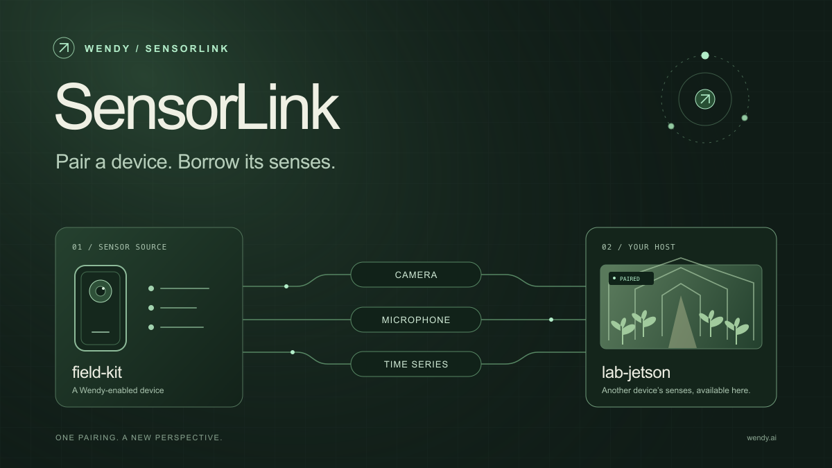
SensorLink: Pair a Device. Borrow Its Senses.
Give your Wendy host the eyes and ears of another device. SensorLink brings cameras, microphones, and a shared model for time-series sensors into a familiar pairing workflow.
Wendy Labs - Wendy Labs Team
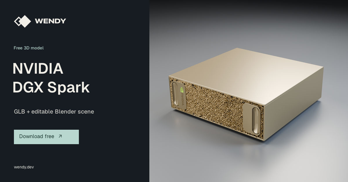
Free NVIDIA DGX Spark 3D model
Download our free NVIDIA DGX Spark 3D model as a GLB or an editable Blender scene with studio lighting, materials, and cameras. No signup required.
Wendy Labs - Wendy Labs Team
Start with one device. Close the loop around it.
Use WendyOS on your hardware or add Wendy Agent to an existing Linux or Apple Silicon Mac. Connect sensors, run your code, and carry what you learn into the next release.